Many phenomena in various science fields are mathematically expressed by using the well-known evolution equations. The diffusion equation is one of them, and mathematically corresponds to the Markov process in relation to the normal distribution rule.

**—Wikipedia: Diffusion equation

A. Standard diffusion equation

Standard diffusion equation is a simplistic second order partial differential equation written as:

\[
\begin{equation}
\frac{\partial \rho(x, t)}{\partial t}
= D \frac{\partial^2 \rho(x, t)}{\partial x^2}
\end{equation}
\]

A1. Finite difference method for time and space

Finite difference of time:

\begin{equation}
\frac{\partial\rho}{\partial t} (x_i,t_j) = \frac{\rho(x_i, t_j + \Delta t) - \rho(x_i, t_j)}{\Delta t} + \mathcal{O}(\Delta t)
\end{equation}

Finite difference of space:

\[
\begin{equation}
\frac{\partial^2\rho}{\partial x^2} (x_i,t_j) = \frac{\rho(x_i+\Delta x,t_j) - 2\rho(x_i,t_j) + \rho(x_i-\Delta x,t_j)}{dx^2} + \mathcal{O}(\Delta x^2)
\end{equation}
\]

A2. Explicit scheme (forward time)

Apply equation(2) and (3) to equation(1), and let \(\rho_{i,j} = \rho(x_i,t_j)\), we get the expression of forward time evolution

\[
\begin{align}
&\ \frac{\rho_{i,j+1} - \rho_{i,j}}{\Delta t} = D \frac{\rho_{i+1,j} - 2\rho_{i,j} + \rho_{i-1,j}}{\Delta x^2} \\
&\Rightarrow \rho_{i,j+1} = (1 - 2\lambda) \rho_{i,j} + \lambda (\rho_{i+1,j} + \rho_{i-1, j})
\end{align}
\]

where \[\lambda=\frac{D \cdot \Delta t}{\Delta x^2}\].
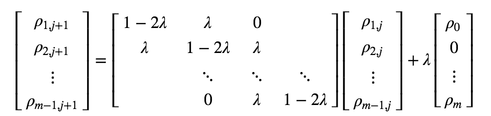
Rewrite this in matrix form,

\[
\begin{equation}
\vec{\rho}_{i, j+1} = A \vec{\rho}_{i, j} + R(\text{accounts for boundary conditions})
\end{equation}
\]

Supplemented by initial condition: \( \rho_{i,0} = \rho(x_i)\),
and Boundary conditions: \( \rho_{0,j} = \rho_0\), \( \rho_{m,j} = \rho_m\), we can solve it like this:

*Sovling an example system with initial value of \(\rho_{center}=1.0\) at center and boundary conditions with \(\rho_L = \rho_R = 0\).

A3. Implicit scheme (backward time)

In implicit scheme, time evolves backwards.

\[
\begin{align}
&\ \frac{\rho_{i,j} - \rho_{i,j-1}}{\Delta t} = D \frac{\rho_{i+1,j} - 2\rho_{i,j} + \rho_{i-1,j}}{\Delta x^2} \\
&\Rightarrow (1 + 2\lambda) \rho_{i,j} - \lambda (\rho_{i+1,j} + \rho_{i-1, j}) = \rho_{i,j-1}
\end{align}
\]

where \[\lambda=\frac{D \cdot \Delta t}{\Delta x^2}.\]
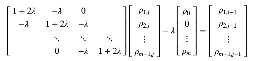
Rewrite this in matrix form,

\[
\begin{equation}
A \vec{\rho}_{i, j} - R = \vec{\rho}_{i, j - 1}
\end{equation}
\]

Supplemented by initial condition: \( \rho_{i,0} = \rho(x_i)\),
and Boundary conditions: \( \rho_{0,j} = \rho_0\), \( \rho_{m,j} = \rho_m\), we can solve it like this:

*Sovling an example system with initial value of \(\rho_{center}=1.0\) at center and boundary conditions with \(\rho_L = \rho_R = 0\).

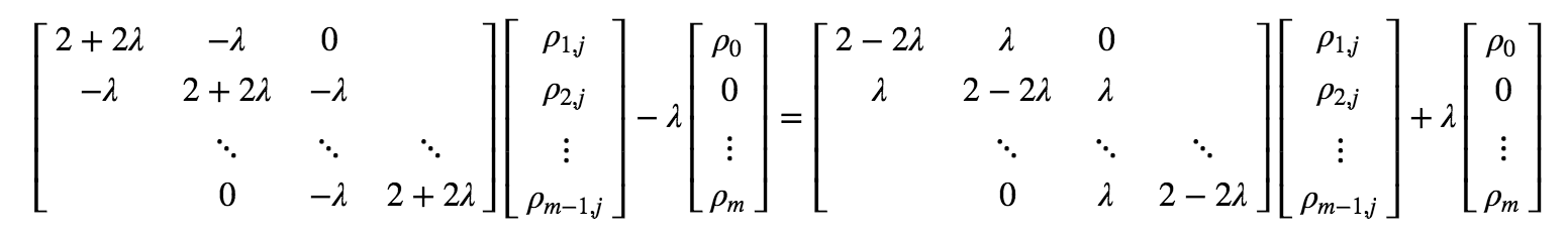
A4. Crank-Nicolson scheme

In Crank-Nicolson scheme, we take the average of explicit scheme and implicit scheme.

\[
\begin{align}
&\ \frac{\rho_{i,j + 1} - \rho_{i,j}}{\Delta t} = \frac{D}{2} ( \frac{\rho_{i+1,j} - 2\rho_{i,j} + \rho_{i-1,j}}{\Delta x^2} + \frac{\rho_{i + 1,j + 1} - 2\rho_{i,j + 1} + \rho_{i - 1,j + 1}}{\Delta x^2} ) \\
&\Rightarrow (2 + 2\lambda) \rho_{i,j + 1} - \lambda (\rho_{i+1,j + 1} + \rho_{i-1, j + 1}) = (2 - 2\lambda) \rho_{i,j} + \lambda (\rho_{i+1,j} + \rho_{i-1, j})
\end{align}
\]

where \[\lambda=\frac{D \cdot \Delta t}{\Delta x^2}\].
Rewrite this in matrix form,

\[
\begin{equation}
A \vec{\rho}_{i, j + 1} - R = B \vec{\rho}_{i, j} + R
\end{equation}
\]

Supplemented by initial condition: \( \rho_{i,0} = \rho(x_i)\),
and Boundary conditions: \( \rho_{0,j} = \rho_0\), \( \rho_{m,j} = \rho_m\), we can solve it like this:

Solvlng an example system with initial value of \(\rho_{center}=1.0\) at center and boundary conditions with \(\rho_L = \rho_R = 0\).

B. Solving diffusion equation with a potential profile.

\[
\begin{equation}
\frac{\partial \rho(x, t)}{\partial t}
= D \frac{\partial}{\partial x}[ \frac{\partial \rho(x, t)}{\partial x} + \frac{1}{k_BT} \frac{\partial U(x)}{\partial x}\rho(x,t)] = D \frac{\partial^2 \rho(x, t)}{\partial x^2} + \frac{D}{k_BT} \cdot U^{\prime}(x) \cdot \frac{\partial \rho(x, t)}{\partial x} + \frac{D}{k_BT} U^{\prime \prime}(x) \rho(x, t)
\end{equation}
\]

The finite difference in Crank-Nicolson scheme for the above equation is:

\[
\begin{align}
&\ \frac{\rho_{i,j + 1} - \rho_{i,j}}{\Delta t} = \frac{D}{2} ( \frac{\rho_{i+1,j} - 2\rho_{i,j} + \rho_{i-1,j}}{\Delta x^2} + \frac{\rho_{i + 1,j + 1} - 2\rho_{i,j + 1} + \rho_{i - 1,j + 1}}{\Delta x^2} ) + \frac{D \cdot U^{\prime}(x_i)}{2 k_BT} (\frac{\rho_{i + 1,j + 1} - \rho_{i - 1,j + 1}}{2 \Delta x} + \frac{\rho_{i + 1,j} - \rho_{i - 1, j}}{2 \Delta x}) + \frac{D \cdot U^{\prime \prime}(x_i)}{2 k_BT} (\rho_{i,j + 1} + \rho_{i,j}) \\
&\Rightarrow (2 + 2\lambda + \tau_i) \rho_{i,j + 1} + (\eta_i - \lambda)\rho_{i+1,j + 1} - (\lambda + \eta_i) \rho_{i-1, j + 1} = (2 - 2\lambda - \tau_i) \rho_{i,j} + (\lambda - \eta_i) \rho_{i+1,j} + (\lambda + \eta_i) \rho_{i-1, j}
\end{align}
\]

where \(\lambda=\frac{D \cdot \Delta t}{\Delta x^2}\), \(\eta_i = - \frac{D \cdot \Delta t}{2 k_BT \Delta x} \cdot U^{\prime}(x_i)\), \(\tau_i = - \frac{D \cdot \Delta t}{k_BT} \cdot U^{\prime \prime}(x_i)\).

Rewrite this in matrix form,

\[
\begin{equation}
A \vec{\rho}_{i, j + 1} - R = B \vec{\rho}_{i, j} + R
\end{equation}
\]

Supplemented by initial condition: \( \rho_{i,0} = \rho(x_i)\),
and Boundary conditions: \( \rho_{0,j} = \rho_0\), \( \rho_{m,j} = \rho_m\), we can solve it like this:

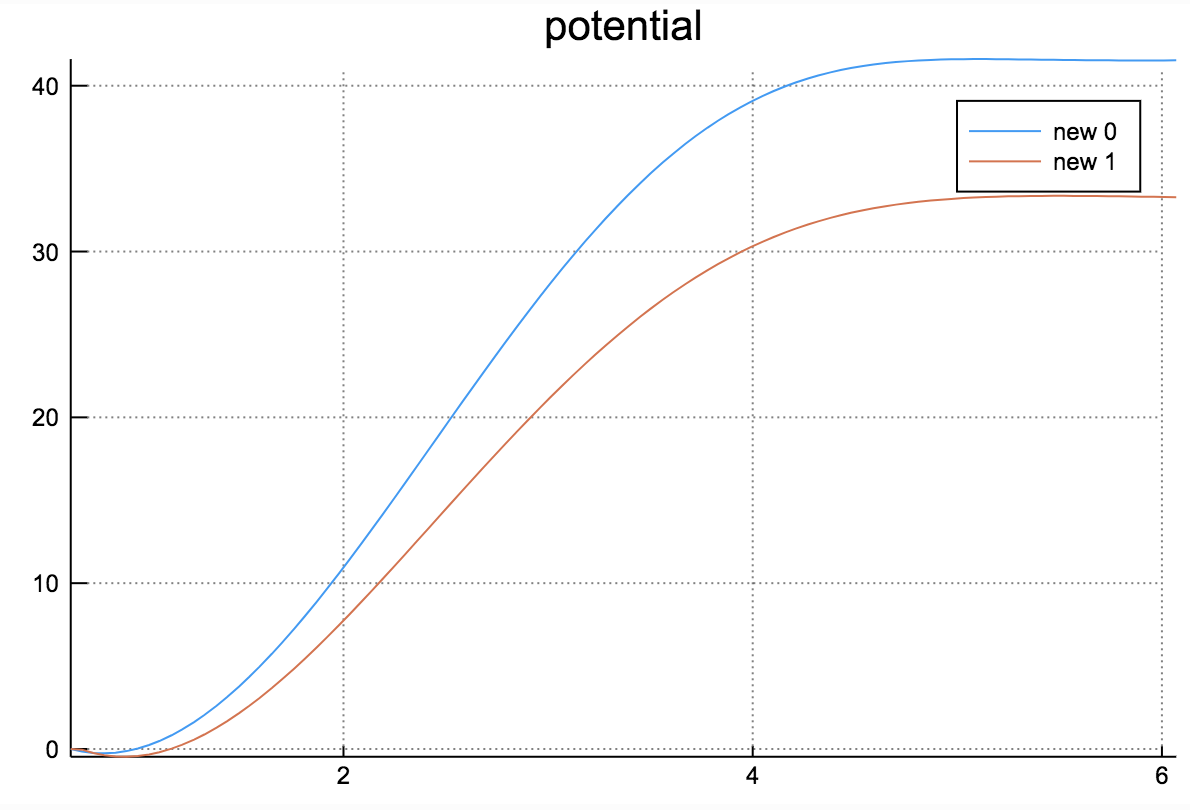
Solving an example system with initial value of \(\rho=1.0\) at \(x=30 \unicode{x212B}\) and boundary conditions with \(\rho_L = \rho_R = 0\) using the potential profile of \(n_w = 0\).

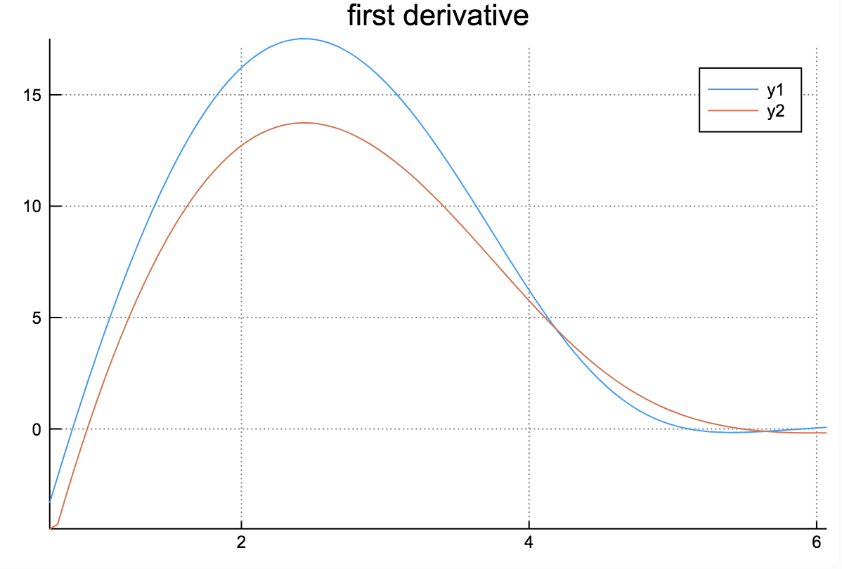
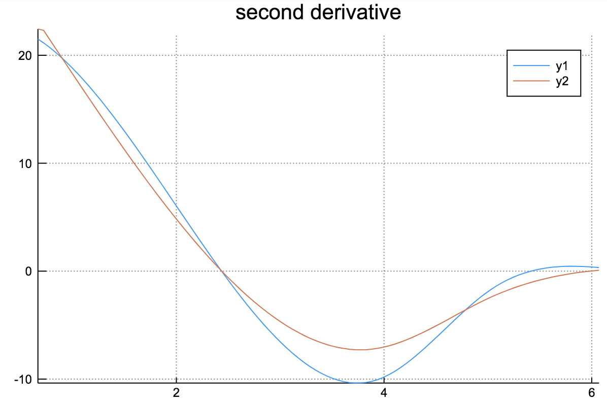
Potential used in this example and its derivatives are as follows:

C. Solving coupled diffusion equations with potential profiles and reactions.

When reaction terms are added to the equation(16), equations corresponding to different \(n_w\) become coupled equations:

\[
\begin{equation}
\begin{cases}
\frac{\partial \rho_0(x, t)}{\partial t}
= D \frac{\partial}{\partial x}[ \frac{\partial \rho_0(x, t)}{\partial x} + \frac{1}{k_BT} \frac{\partial U_0(x)}{\partial x}\rho_0(x, t)] - [k_{0 \to 1} + k_0^{wf}(x)]\rho_0(x, t) + k_{1 \to 0}\rho_1(x, t) \\
\frac{\partial \rho_1(x, t)}{\partial t}
= D \frac{\partial}{\partial x}[ \frac{\partial \rho_1(x, t)}{\partial x} + \frac{1}{k_BT} \frac{\partial U_1(x)}{\partial x}\rho_1(x, t)] - [k_{1 \to 2} + k_{1 \to 0} + k_1^{wf}(x)]\rho_1(x, t) + k_{2 \to 1}\rho_2(x, t) + k_{0 \to 1}\rho_0(x, t) \\
\frac{\partial \rho_2(x, t)}{\partial t}
= D \frac{\partial}{\partial x}[ \frac{\partial \rho_2(x, t)}{\partial x} + \frac{1}{k_BT} \frac{\partial U_2(x)}{\partial x}\rho_2(x, t)] - [k_{2 \to 3} + k_{2 \to 1} + k_2^{wf}(x)]\rho_2(x, t) + k_{3 \to 2}\rho_3(x, t) + k_{1 \to 2}\rho_1(x, t) \\
\vdots \\
\vdots \\
\frac{\partial \rho_{n-1}(x, t)}{\partial t}
= D \frac{\partial}{\partial x}[ \frac{\partial \rho_{n-1}(x, t)}{\partial x} + \frac{1}{k_BT} \frac{\partial U_{n-1}(x)}{\partial x}\rho_{n-1}(x, t)] - [k_{n-1 \to n} + k_{n-1 \to n-2} + k_{n-1}^{wf}(x)]\rho_{n-1}(x, t) + k_{n \to n-1}\rho_n(x, t) + k_{n-2 \to n-1}\rho_{n-2}(x, t) \\
\frac{\partial \rho_n(x, t)}{\partial t}
= D \frac{\partial}{\partial x}[ \frac{\partial \rho_n(x, t)}{\partial x} + \frac{1}{k_BT} \frac{\partial U_n(x)}{\partial x}\rho_n(x, t)] - [k_{n \to n-1} + k_n^{wf}(x)]\rho_n(x, t) + k_{n-1 \to n}\rho_{n-1}(x, t)
\end{cases}
\end{equation}
\]

Let \(\rho_{i,j}^k = \rho_k(x_i,t_j)\), the finite difference in Crank-Nicolson scheme for \(n_w = k\) is:

\[
\begin{align}
&\ \frac{\rho_{i,j + 1}^k - \rho_{i,j}^k}{\Delta t} = \frac{D}{2} ( \frac{\rho_{i+1,j}^k - 2\rho_{i,j}^k + \rho_{i-1,j}}{\Delta x^2} + \frac{\rho_{i + 1,j + 1} - 2\rho_{i,j + 1} + \rho_{i - 1,j + 1}}{\Delta x^2} ) + \frac{D \cdot U_k^{\prime}(x_i)}{2 k_BT} (\frac{\rho_{i + 1,j + 1}^k - \rho_{i - 1,j + 1}^k}{2 \Delta x} + \frac{\rho_{i + 1,j}^k - \rho_{i - 1, j}^k}{2 \Delta x}) + \frac{D \cdot U_k^{\prime \prime}(x_i)}{2 k_BT} (\rho_{i,j + 1}^k + \rho_{i,j}^k) - \frac{k_{k \to k-1} + k_{k \to k+1} + k_k^{wf}(x_i)}{2} (\rho_{i,j+1}^k + \rho_{i,j}^k) + \frac{k_{k-1 \to k}}{2} (\rho_{i,j+1}^{k-1} + \rho_{i,j}^{k-1}) + \frac{k_{k+1 \to k}}{2} (\rho_{i,j+1}^{k+1} + \rho_{i,j}^{k+1})\\
&\Rightarrow (2 + 2\lambda + \tau_i^k) \rho_{i,j + 1}^k + (\eta_i - \lambda)\rho_{i+1,j + 1}^k - (\lambda + \eta_i^k) \rho_{i-1, j + 1}^k + \xi_i^k \rho_{i,j + 1}^k - \zeta^k \rho_{i,j + 1}^{k+1} - \kappa^k \rho_{i,j + 1}^{k-1} = (2 - 2\lambda - \tau_i^k) \rho_{i,j}^k + (\lambda - \eta_i^k) \rho_{i+1,j}^k + (\lambda + \eta_i^k) \rho_{i-1, j}^k - \xi_i^k \rho_{i,j + 1}^k + \zeta^k \rho_{i,j + 1}^{k+1} + \kappa^k \rho_{i,j + 1}^{k-1}
\end{align}
\]

where

\[
\begin{align}
&\lambda=\frac{D \cdot \Delta t}{\Delta x^2} \\
&\eta_i^k = - \frac{D \cdot \Delta t}{2 k_BT \Delta x} \cdot U_k^{\prime}(x_i) \\
&\tau_i^k = - \frac{D \cdot \Delta t}{k_BT} \cdot U_k^{\prime \prime}(x_i) \\
&\xi_i^k = (k_{k \to k+1} + k_{k \to k-1} + k_k^{wf}(x_i)) \Delta t \\
&\zeta^k = k_{k+1 \to k} \Delta t \\
&\kappa^k = k_{k-1 \to k} \Delta t
\end{align}
\]

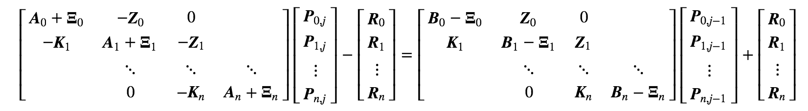
We further define following \((m-1) \times (m-1)\) matrices:

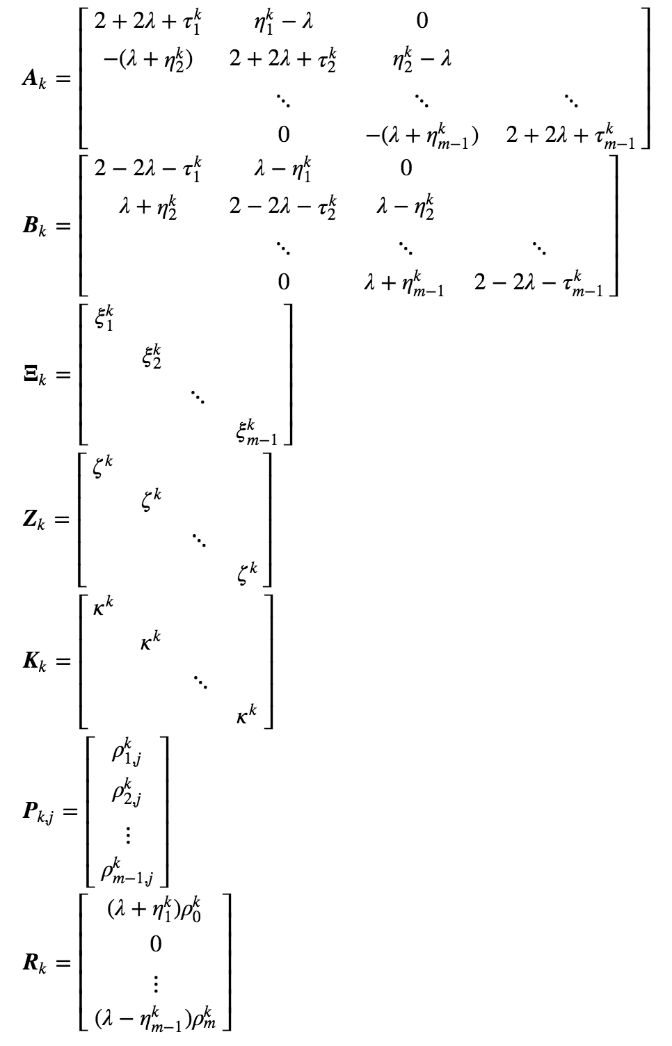
Rewrite in matrix form,

Solving an example system with initial value of \(\rho=1.0\) at \(x=40 \unicode{x212B}\) for all \(n_w=0:9\) and boundary conditions with \(\rho_L = \rho_R = 0\) using the potential profile of \(n_w = 0\).

The above example calculations are produced using Julia 6.0 with matplotlib. You can find the example jupyter notebook file HERE.